Do you have a large set of data that you need to lookup for values? VLOOKUP in Excel can help you cut down the time to search for values. This article will help learn how to use VLOOKUP in Excel.
Do you want to level up your Excel skills and be more productive at the same time? Then master VLOOKUP in Excel. VLOOKUP is an intermediary formula that helps you easily find and return value for a range of data in a row. After reading this article, you should learn how to use the VLOOKUP function. Most importantly, you should be able to understand the concept behind the formula so you will understand by heart how it works.
How to Use VLOOKUP in Excel
The next sections will guide you on what is VLOOKUP, how to use the formula, and how the formula works so you can fully understand and maximize the use of the formula.
What is VLOOKUP?
VLOOKUP in Excel allows you to easily lookup row values in a specific table. VLOOKUP eliminates the manual finding of data in a given set of rows. Let’s take a look at the table below as an example.
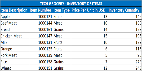
The item inventory table above can give answers to these following questions:
• What is the price per unit of milk?
• How many apples are there?
• What is the item type of pork?
• Can you tell what is the item number of orange and wheat?
• What is the price per unit of bread?
Based on the item inventory table, you can say that the price per unit of milk is $10 and that there are 145 apples in the inventory. The other questions can be answered simply by looking at the table above.
Manual looking up for the values would be easy since the available data is only minimal. But what if there are thousands of items and at least 50 rows per item? How can you look for specific data of each item? In situations where there are too many data to do a manual vertical lookup, VLOOKUP in Excel can help be an effective tool.
What is the VLOOKUP Formula?
This is the VLOOKUP formula:
The VLOOKUP formula is broken down into:
• VLOOKUP is the function you want to execute.
• Lookup value is your reference value.
• Table array is the column range where you want to do the lookup. Take note that the range should start at the • column where the lookup value is located.
• Column index number is the number of columns from the first column where the resulting data is located.
• Range lookup is optional where you can enter TRUE if you want to do an approximate match and FALSE if you want to do an exact match.
Let’s look at the table again:

Now, going back to this question: What is the price per unit of milk? The answer is obviously 10.
To do the same question using the VLOOKUP function, we will apply the formula:
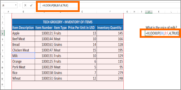
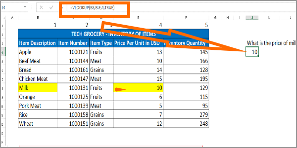
Excel will return the value based on your formula. In this case, Excel will return the value of 10.
Understanding the VLOOKUP Formula
To ensure that you fully understand the VLOOKUP formula, let’s use the question on the price per unit of the milk. Let’s look at the table again:

Using the VLOOKUP formula:
Now, let’s relate it to the question: What is the price per unit of milk? The answer is 10.
VLOOKUP is simply WHAT, WHERE, and HOW MANY?
• What? Milk (B8)
• Where? Columns B to F
• How many columns? 4 columns
Compare the WHAT-WHERE-HOW MANY above to the formula:
Now, what do we get? A 10!

VLOOKUP is a helpful tool to cut down the process of manually looking for the data. All you need to do is understand the core ideas behind the formula. Once you understand the basics of VLOOKUP in Excel you will find a lot of ways and situations where you can use the function to your advantage.
You just learned how to use the VLOOKUP in Excel. If you have questions about any of the information presented in this article, let us know in the comments section.

