You can calculate percentage in Excel through many different methods. Some involve formatting cells and use of complex formulae, while others do not. Our main focus will be on the latter.
I know how most tutorials entangle you in complexities. Calculating something as simple as a percentage shouldn’t be a mentally exerting process.
That’s why this tutorial will teach you how to calculate percentage in Excel with commanding ease. Whether it’s a percentage increase for a list of grocery items or a % decrease in sales tax you’re computing, we will make it as easy as ABC.
How to Calculate Percentage In Excel
In this example, we will calculate the absolute percentage and % increase and decrease for the number 100. This is just to show you how things work. You can input any other value in the cell references and follow our method to get your intended results.
Finding the Absolute Percentage
1. Click an empty cell.
2. Start your formula with “=”.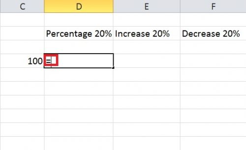
3. Click the cell reference you want to compute the percentage of. In this case, it’s cell reference C4. You can also manually type its name. 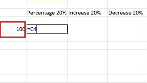
Multiply cell reference with your intended percentage (C4*20%).
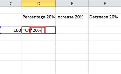
4. Press Enter to get your result.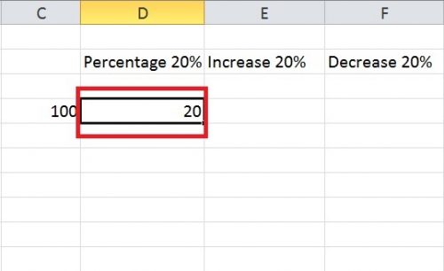
Finding Percentage Increase
1. Do steps 1 and 2 mentioned above.
2. Insert the formula : = C4+C4*20% instead of = C4*20%.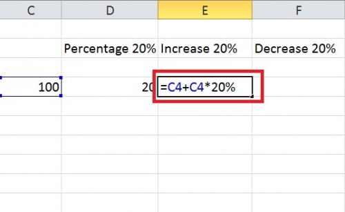
Note: You can change this formula according to your situation. For instance, if you the number you want the percentage calculated for is in another cell reference, modify the formula keeping that cell reference in mind.
3. Press Enter.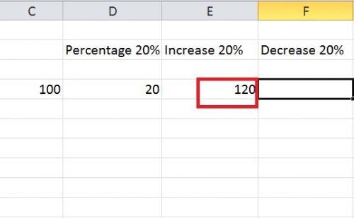
Finding Percentage Decrease
1. Follow the Steps 1 and 2 of finding absolute percentage.
2. Insert the formula: = C4-C4*20%.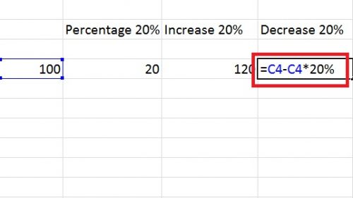
3. Press Enter.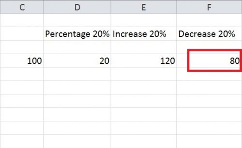
Read More: How to Write a Custom Function in Excel
Calculating Percentages for a Column of Numbers
If you’r working with many numbers, just stretch the column with the computed percentage downward. It will automatically fill in the percentages for the rest of the numbers.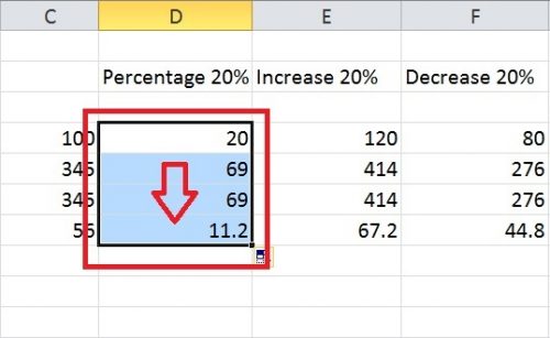
Formatting Cells to Calculate percentages
You can also format cells to modify percentages. For instance if you want your percentage to be a multiple of 100, here’s what you have to do.
1. Right click the cell reference you wish to format and select format cells. In this case, I’m formatting the cell reference D2.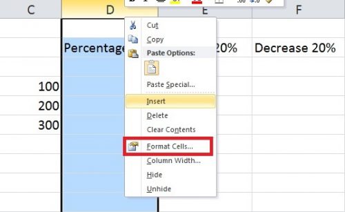
2. Select percentage from the side menu and the number of decimal points you want your percentage to be a multiple of.
3. Press Enter.
So, this is how to format percentages in Excel with exceptional convenience. It doesn’t require sophisticated formulae or conditional formatting of cells, or anything of the sort. Just a few steps and you have yourself a swift answer.
Finding Percentage Change For Two Different Values
Sometimes, none of the above examples apply to you. You’re actually interested in calculating percentage Change for two different values in the two different cells. For that, follow the Youtube tutorial given below to guide you each and every step of the way.
Learning how to calculate percentage change in Excel through text is hard and often confusing. It’s something I wouldn’t recommend. And that is why I’ve refrained from outlining it here.

