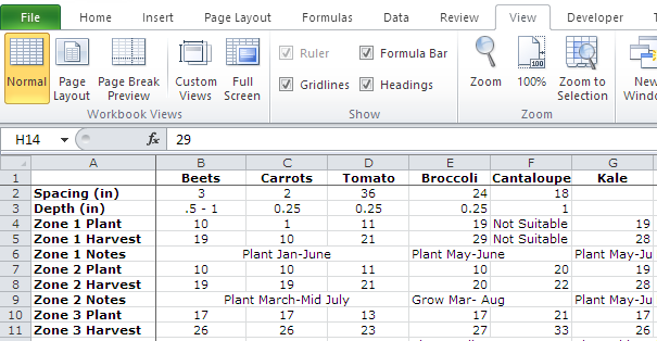
Working with a large set of data in Microsoft Excel can be tricky. It is particularly aggravating when several columns or rows of data are similar, so you have to keep jumping back to the header to remember what you are viewing. A good solution to this is to freeze columns, rows, or both so that they stay displayed on your screen while you scroll through the rest of your data. Here’s how to do it.
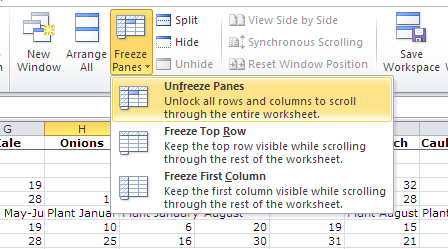
If you want to freeze the top row or first column, just go to View> Freeze Panes, and then click on either Freeze Top Row or Freeze First Column.
If you want to freeze rows AND columns at the same time, follow the steps below.
Freeze Rows AND Columns at the Same Time
1.Select the first cell that you want to be unfrozen. That means that every cell above it and to the left of it will be frozen. In my example, I want to freeze the top row and the first column, so I click on cell B2. If I had selected B3, the top two rows and first column would be frozen. 
2.Go to the View tab, and click Freeze Panes.
3.Lines will appear on your spreadsheet separating out the frozen columns and rows from the scrollable part of your spreadsheet. 
4.If you want to turn off your frozen rows and columns, go back to View>Freeze Panes and select Unfreeze Panes.
Here are some tips for effective freezing:
- You cannot freeze rows or columns in the middle of the sheet. They have to be at the top or left.
- You can freeze multiple rows, multiple columns, or a combination of both
- You will need to use Freeze Panes to freeze multiple rows or columns. Select the rows/columns by clicking on the header number/letter of the first row/column to freeze, and then click the last one while holding down the Shift key on your keyboard.
- The Freeze Panes button will be grayed out if you are editing a cell.


