Did you create a spreadsheet and realize that you got the layout mixed up? Did you receive a table or a chart through your email, but you need to reformat it? Excel’s Transpose option will allow you to fix your charts easily.
When to put data into rows or columns is debatable. When receiving a spreadsheet with data entered incorrectly, many users will delete the columns and manually re-enter them in rows. Obviously, this method is slow and painful. The faster way to fix your tables is by using the Transpose feature. By using this feature you can convert your column-based chart to simple table rows.
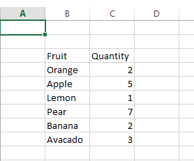
1.Below is a column-formatted data. Select the whole table.
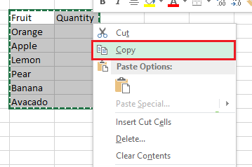
2.With the data highlighted, right-click on it, and click Copy.
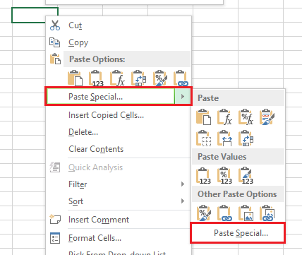
3.Right-click on an empty cell, and select Paste Special and then Paste Special… again.
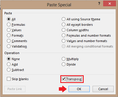
4.Under Paste Special, select the check box next to Transpose , and click OK.
Through these steps you will be left with your reformatted table.


