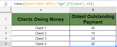
You can use Google Sheets DMAX function to find the maximum value in a range based on some criteria. For example, if you have a table of data with outstanding payments you are owed from each of your clients, you can use DMAX to find the oldest of the outstanding payments for each client.
In my example, I will be using this source data in Sheet 2. 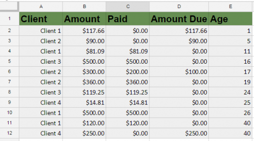
I want to create a summary in Sheet 1 where I look up the oldest outstanding payment that each client owes me.
1.First, I need to set up my table in Sheet 1. I can set up my list of client names by typing them into column A or by using the unique function.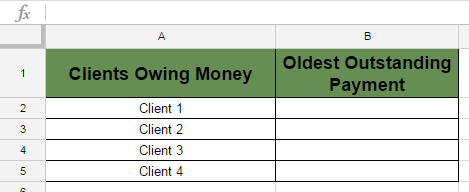
2.Type in the following:
=dmax(
Then use your mouse to highlight the entire database of your source data that contains the columns you will be using – including headers. In my case, it is Sheet2!A1:F12. If you are going to be copying this formula down (as I am to look up all four clients), then hit F4 on your keyboard to change this from a relative to absolute formula, which will look like Sheet2!$A$1:$F$12.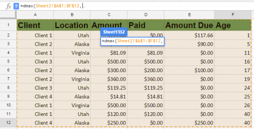
3.Type in a comma, and then type in field or the column header name from the database from which you want to return values. Include quotes around the text. In my case, that is “Age”.
4.Type in a comma, followed by curly brackets {}. The criteria used to sort through the max will go inside of the curly brackets. First comes the database column, then a semicolon, and then the criteria to which I want to compare it. In my case, that is {“Client”; A2}. (A2 is the filtered client name in Sheet 1 next to where I am typing in the formula.) Remember to use quotes around the header name. Close the parenthesis, hit enter, and you will see the maximum age for the client that matches A2.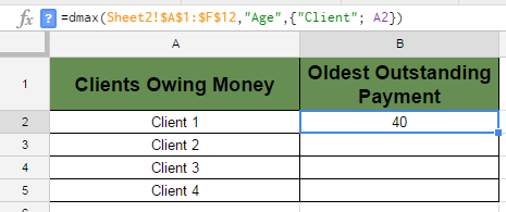
5.Click on cell B2, and then click on the bottom right corner and drag it down to B5. This will copy the formula into those cells to check for the other clients. Because you used an absolute reference for the database in Step 1 and a relative reference for the criteria in Step 4, you do not need to change anything with the formulas.