I recently worked on a spreadsheet with a table that was populated using the filter function. This meant that I did not know how many rows would be included in my table: It would dynamically update as the source data changed. I wanted to apply some formatting to the table so that it would look better than straight text. I achieved this by applying conditional formatting to all the cells that could be included in the table. The conditional formatting was set to shade the cells that were not blank to make my table look more cohesive. This tutorial explains how to format cells that are not blank when using Google Sheets.
1.Highlight the range of cells to which you want to apply the conditional formatting. Go to Format>Conditional Formatting.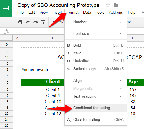
2.The Conditional format rules panel appear on the right side of the screen. Click Add new rule.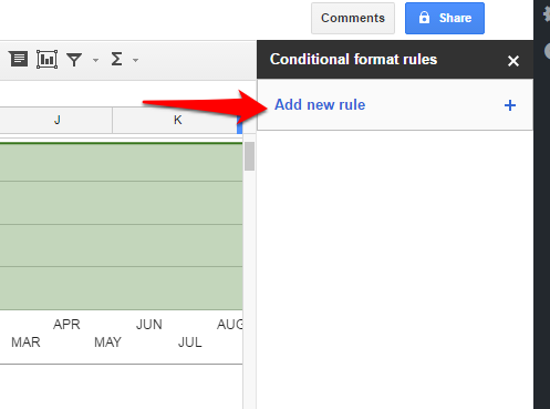
3.Check to see if the ranges in the Apply to range box are correct. If not, click in that area to type in the correct range or select it. You can also add multiple ranges to which the rule applies. This is helpful because it means that, once you set up this rule, you can use it throughout your workbook by adding ranges to the rules.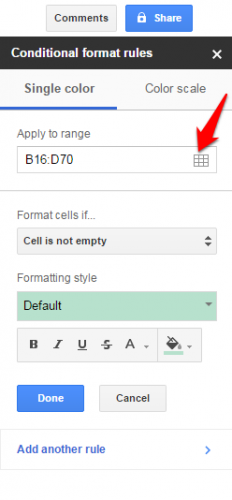
4.In the next box, choose Cell is not empty from the list of options.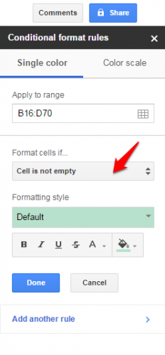
5.Now set the format options. You can choose a default option or manually select the font color, cell background color, and text effects (bold, italics, underline, and strike through). Unfortunately, you cannot currently add or change borders using conditional formatting in Google Sheets. 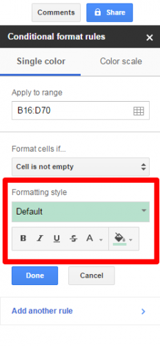
6.Click Done to hide the conditional formatting panel when you are satisfied with the formatting. 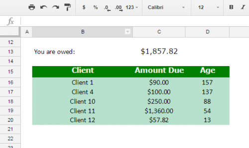
Note that, although I applied the formatting rule to a range that included both blank and non-blank cells, only the non-blank cells were formatted. This is perfect for situations like mine where my spreadsheet needs to dynamically adapt as new data is entered.
Do you have other applications where you need to format non-blank cells? Comment below to help the community out!

