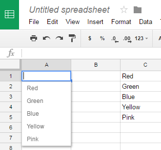
Creating a drop down list in Google Sheets using data validation is pretty simple. When a cell has data validation applied to it, people who use your spreadsheet will be able to select a value for the cell based on a list that you create. You can refer to the content selected in other cells, which gives you a lot of freedom for dynamic spreadsheets.
In this example, I will make a drop down list in Cell A1 that will contain a list of colors.
1.Create a list of the items you want included in your drop down list. This list can be placed anywhere in the workbook, even on a different sheet. I placed my list in cells C1:C5 of the same sheet where the drop down will be. Next, click on the cell that you want to turn into a drop down list. 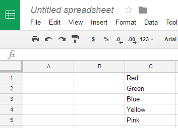
2.Go to Data>Validation.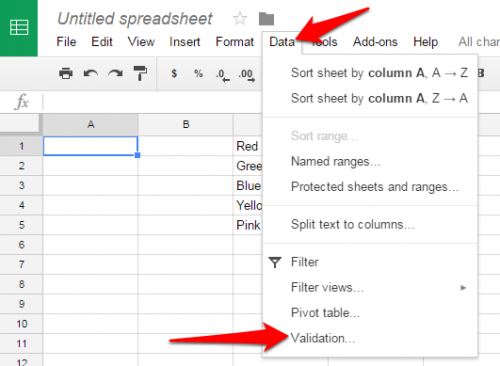
3.The Cell range should already be set to the cell where you want to create the drop down menu if you had it selected before you opened up the data validation dialog box. If not, type in a new cell reference, or click on the grid to the right of it to select it from your workbook. Set the Criteria to be the cells containing your list. You can do this by typing in the cell reference or by clicking on the grid and then highlighting the cells you want included. Click Save.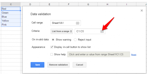
Note: The On invalid data options determine if you will allow users of your spreadsheet to override your drop down list with whatever they want to type in. “Reject input” will result in users getting an error message if they type anything other than an approved item, while “Show warning” will result in an orange tick mark in the corner of the cell if the user types in their own content.
4.Now you will notice an unobtrusive down arrow at the edge of the cell with the newly added validation. 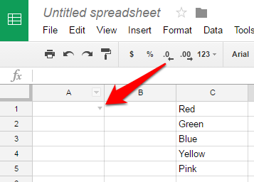
5.Click on the cell to see the list, and click on an item to populate the cell with that item.
