The Unique function in Google Sheets makes it simple to create a list of only unique values from another list. One of the most useful aspects of the Unique function is that you type the formula into one cell, and it will fill in the cells beneath it with all the unique values in the range you specified. Interestingly, the formula only exists in the top cell. There is no need to copy down the formula or anything else. Just make sure that you have adequate blank cells adjacent to where you type the formula for all the items in the list. This tutorial contains the steps you need to use the Unique function in Google Sheets.
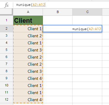
1.In the cell where you want to begin your list, type in the following:
=unique(
Then drag your mouse around the range that has all the values where you want to pull unique values. Your range can be on another tab, and it can consist of multiple rows and columns. Hit Enter.

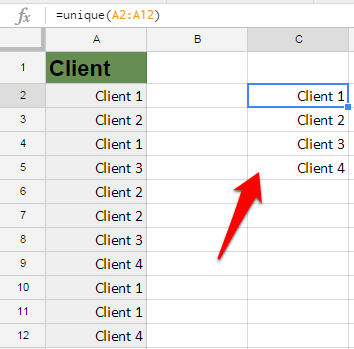
2.In this example, the formula returns the four unique client names from the range “A2:A12” in four adjacent cells. If you look at cells C3, C4, and C5, there will be no formula – just the values created by the formula in cell C2.

3.If your source range is listed in a row instead of a column, Google Sheets Unique will return the data in a row as well. 
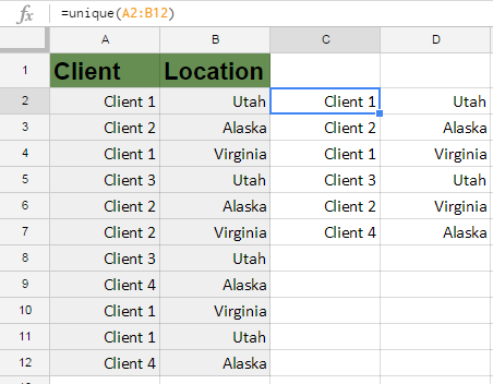
4.If you change the range to include two adjacent rows or columns, the Unique function will return values that are unique between the selected columns. You will need to leave room for the function to return as many columns as you selected in your source range. Note how, in this example, Clients 1 and 2 each appear twice in the list created by the Unique function. This is because there were two different locations tied to the client.
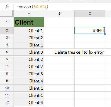
5.If you get a #REF! error, it is probably because you did not leave enough space for the filter function to fill in all the rows it wants to return. You need to leave plenty of space for it to do its thing. You also get this error if you try to type over or delete any of the result cells created by the function.


